Mixed Signal & Domain Simulation for Embedded Worlds

Mixed-domain Simulation and Visualization of a Two Wheel Robot with Blender Open-source Software¶

In the Conceptual Simulation of Digital Sine Generator from Eagle we have learnt about basic principles how to combine analog and digital worlds in simulation together by using open-source tools and the very popular Eagle CAD. In this article you will learn how to use ngSpice and its’ Eagle extension to do a conceptual simulation of a two wheel robot and visualize its movement using the open-source blender, a 3D modeling and animation software.

Uros Platise, 22. August 2017

Mechatronics, one of the fastest growing area, is an interdisciplinary area that describes simple electro-mechanical devices as well as complex robotics systems. Designing such systems calls for a system level simulation in which electronic and mechanical domains could be simulated together. ngSpice can be seen as general purpose multi-dimensional differential equation solver and as such it can do just anything if one knows to describe. In this article we are going to model a simple two wheel robot, stimulate forces on its two wheels and observe it’s dynamics. Furthermore we are going to visual robots movements with the popular blender 3D modeling and animation software and move blender object around.

The Tools¶

Besides the tools mentioned under the Conceptual Simulation of Digital Sine Generator from Eagle we additionally need:

Blender ¶

Blender is a free and open source 3D creation suite. It supports the entirety of the 3D:

pipeline—modeling,
rigging,
animation,
simulation,
rendering,
compositing,
motion tracking,
even video editing and game creation.

Mechanical Model and Simulation of a Two Wheel Robot¶

Modeling of a mechanical systems is in great extend covered by universities, their books as is for example this book on Modeling of Mechanical Systems for Mechatronics Applications from University of Texas. Limitations apply similarly as in the cases of electronics devices, and there are plenty of studies how to enhance mathematical models for each specific group of applications.

Nevertheless we shall model a simple two wheel vehicle which can with some intelligence turn into a robot.

Model of the Two Wheel Vehicle¶

Let’s assume our two wheel vehicle is of form of a box with two wheels as shown below (top-view):

Each wheel is powered by a motor to stimulate forces F1 for the first motor and F2 for the second. Note that forces are in practice directly proportional to the current of the electric motor. In reverse direction to the motor, there is a friction force Ft1 contrarily the F1, and Ft2 the F2, proportional to the speed of the wheel $F_t = k v$ .

Observing the robot (cube) from its central point it translates forward and backward only if both forces are of same value, otherwise their difference causes a momentum $M = r F_p$ that changes movement for some angle $dp/dt$ .

So we have forces that stimulate translational movement:

$F_s = F_1 + F_2 - k_1 v_1 - k_2 v_2$

The speeds $v_1$ and $v_2$ are relative to wheels, so any imbalance in $F_1$ and $F_2$ would cause rotation, so speed as seen by the first wheel $v_1$ and second $v_2$ is:

$v_1 = v + r dp/dt v_2 = v - r dp/dt$

where p is angle of the robot, and momentum forces that cause robot to turn are:

$F_p = F_1 - F_2 - k_1 v_1 + k_2 v_2$

These equations describe a very basic model of a vehicle.

Drawing a Model within Eagle¶

From system theory we learnt that linear systems can be modeled using a summer (+) and integrator (1/s), whereas to complicate a bit our module and make it non-linear we are going to add a limiter function to set the friction (sliding) force, so turning $k(v)$ into $limiter(v)$ .

In the Eagle ngSpice Library (ngspice.lbr) you may find similar to Matlab/Simulink like components, provided by the xspice extension in the ngspice. In the previous article Conceptual Simulation of Digital Sine Generator from Eagle we have described how to set values of the user modified parts. Here we may see the block SUM_MT is defined at A8 as pin 1 to have gain +1 and pin 2 has gain -1. The part A6 re-uses this definition by specifying value as SUM_MT# - so note that # at the end to ignore re-definition of the spice model and re-call the one from A8.

The following spice model is built around analog components only, voltages as signals. Nets are labeled to express forces, path, angle, and their derivatives are prefixed with a d character.

To summarize the key forces in the model and test setup:

F1 and F2 represent forces of the two motors, with two voltage pulses as stimulus,
Fs represent the SUM of translation forces in forward and backward direction s
Fp represent the SUM of forces around the central point of the vehicle, and its rotation p

and the outputs:

The s represent movement along the way of the vehicle, however
at angle p, so we transform them into
x and y using the ds and current angle p

Simulation¶

Parameters in the model were randomly chosen so we are not going to dig into numbers in further simulation but rather in the concept of simulation, data export and visualization.

To obtain model’s response let’s run simulation for 10 seconds with stimulus as follows:

first, force is applied to the first motor (F1) for a second, then
after 0.5 second the same amount of force is applied to the second motor (F2) for two seconds.

These can be seen in the chart on the left and besides on the right are accumulative forces are shown that apply on model’s movement as a result of simulation.

Vehicle’s total movement is seen on the left (note that the p is in radians), and translated to the (x,y) coordinate system is seen in the right chart.

Exporting Charts, Schematics and Data¶

A few words about exporting charts and schematics:

The above schematics from Eagle was exported by going to File and Print to PDF. Set the scale factor properly to fit the desired page size and print it. The pdf was then converted using another great tool the Inkscape. Simply open the PDF and use the default parameters in the PDF Import Dialog. In the above example we exported the Eagle onto A4 sheet portrait, and we rotated it inside the Inkscape, and saved file as “Plain SVG”.

The charts are exported from the ngspice using the hardcopy command, or you may use the hardcopy button when using the plot command. For example:

ngspice -> plot fs
ngspice -> hardcopy fs.ps fs

First would show the fs variable on screen and the second would print that same variable to the postscript file: fs.ps. One may want to add a white backgrond instead of black for documenting purposes, for postscript, set the following variable to 1, which sets the background color to obtain charts as seen above.

ngspice -> set hcopypscolor=1

or may select a different font, for example:

ngspice -> set hcopyfont=Arimo

The generated postscript can be converted by using the ps2pdf. One one avoid installing it (anyway it’s a kind of standard tool on linux systems) by using an on-line ps2pdf converter, one may again use inkscape to modify it a bit and save as svg, or one may use a great tool called pstoedit to convert it directly to the svg and many other formats.

One may want to change screen colors by modifying the color0 (background) and color1 (text) as follows:

ngspice -> set color0=rgb:f/f/f
ngspice -> set color1=rgb:0/0/0

Note: colorN settings may interfere with the postscript hcopypscolor and postscript result may not be correct.

The raw simulation data are exported using the ngspice wrdata robot.ssv x y p command which generates a space separated file format in pairs (time, variable). The robot.ssv therefore contains 6 columns in the following order: [time, x, time, y, time, p] as:

00000000e+00  0.00000000e+00  0.00000000e+00  0.00000000e+00  0.00000000e+00  0.00000000e+00
00000000e-05  0.00000000e+00  1.00000000e-05  0.00000000e+00  1.00000000e-05  0.00000000e+00
00000000e-05  0.00000000e+00  2.00000000e-05  0.00000000e+00  2.00000000e-05  0.00000000e+00
00000000e-05  0.00000000e+00  4.00000000e-05  0.00000000e+00  4.00000000e-05  0.00000000e+00
00000000e-05  0.00000000e+00  8.00000000e-05  0.00000000e+00  8.00000000e-05  0.00000000e+00
60000000e-04  0.00000000e+00  1.60000000e-04  0.00000000e+00  1.60000000e-04  0.00000000e+00
20000000e-04  0.00000000e+00  3.20000000e-04  0.00000000e+00  3.20000000e-04  0.00000000e+00
40000000e-04  0.00000000e+00  6.40000000e-04  0.00000000e+00  6.40000000e-04  0.00000000e+00
00000000e-03  0.00000000e+00  1.00000000e-03  0.00000000e+00  1.00000000e-03  0.00000000e+00
00072170e-03  1.87943339e-15  1.00072170e-03  2.69563336e-30  1.00072170e-03  1.87945780e-15
00216509e-03  2.81910668e-14  1.00216509e-03  1.51051916e-28  1.00216509e-03  2.81918236e-14
00296243e-03  5.21424864e-14  1.00296243e-03 -1.02524924e-26  1.00296243e-03  5.21439917e-14
00389075e-03  9.67919710e-14  1.00389075e-03 -6.67916527e-27  1.00389075e-03  9.67950936e-14
...

Visualization of Robot Movements with Blender¶

If you’re completely new to Blender you might find it hard to navigate as there are so many options that you cannot find them unless you really know where they are. Therefore I would suggest you to go through some tutorial as is the Blender Tutorial for Beginners: How To Make A Mushroom to learn navigating for basic usage.

Blender, written in python, offers immense extension capabilities with a very well documented Blender API 2.77.3 or newer about all the methods and data structures accessible from python.

Let’s start Blender and do few steps to make a cube running around.

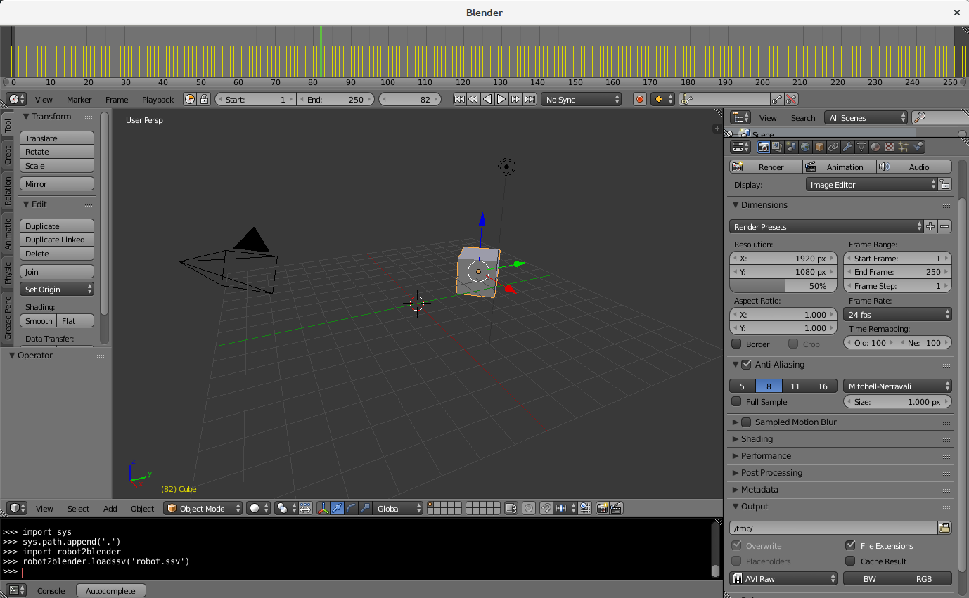
Menu-bars, tool-bars, these are all configurable to represent the most needed tools at a time.

We have set the upper line to be in a Timeline view (click on the left icon besides the View).
The most bottom menu line was set to display Python console.
On the right we have switched to the Render view, we’ve set Frame rate to 50 fps and output file format to the AVI

Each object in Blender has a name, and the default Cube has a name Cube. So for instance to move cube around from python one would write, for example:

bpy.data.objects["Cube"].location[0] = 10

To import ngspice’s output data we prepared robot2blender.py script that reads x,y,p data from given file, skips over-sampled information to 50 fps, and applies it to the Cube.

To use one may need to provide default searching path to the current folder as:

import sys
sys.path.append('.')

and then simply as:

import robot2blender
robot2blender.loadssv('robot.ssv')

We may see how the timeline above got populated with the frames. You may move the green line with the mouse and you shall see the cube moving according to the frame’s defined position and orientation.

To generate AVI video, just press the Animation button as seen in the right toolbar. Blender will start processing frame by frame and output a single AVI file, which result follows:

To convert it to a MP4, a web browser friendly format, use ffmpeg as:

ffmpeg -i blender-robot.avi -c:v libx264 -pix_fmt yuv420p -preset medium -b:v 2600k -movflags +faststart blender-robot.mp4

Conclusion¶

We have learnt the basic steps how to model a mechanical system in ngspice, it’s xspice extension and with the help of Eagle, and ngspice extension for Eagle. Additionally we have learnt some more tips on exporting data and use of blender to visualize movements.

The whole project source files can be downloaded from github.

Continue to The Easiest Way of Simulating C/C++ Code Together with an Analog & Digital Spice Simulation

Download Software	User Guides
Isotel NgSpice Fork \|github\|_	Introduction to Open Source Spice Mixed Signal & Verilog Simulation Conceptual Simulation of Digital Sine Generator from Eagle Mixed-domain Simulation and Visualization of a Two Wheel Robot with Blender Open-source Software The Easiest Way of Simulating C/C++ Code Together with an Analog & Digital Spice Simulation Platise Ferromagnetic (Non-Linear) Model

Download Software

User Guides

Isotel NgSpice Fork

|github|_

Introduction to Open Source Spice Mixed Signal & Verilog Simulation

Conceptual Simulation of Digital Sine Generator from Eagle

Mixed-domain Simulation and Visualization of a Two Wheel Robot with Blender Open-source Software

The Easiest Way of Simulating C/C++ Code Together with an Analog & Digital Spice Simulation

Platise Ferromagnetic (Non-Linear) Model