
Mixed Signal & Domain Simulation for Embedded Worlds
Platise Ferromagnetic (Non-Linear) Model
Represents a novel mathematical model for describing a non-linear characteristics of soft ferromagnetic materials without hysteresis.
Uros Platise, 6th November 2022 and updated on 30th March 2024
In power electronics magnetic materials represent key components for which
curves are typically described with charts. Users then need to re-type the values which simulators and solvers then interpolate them, either with linear or cubic splines. Extra tweaking is needed to ensure monotonically increasing function to avoid local minimums causing divergence. Here another approach is represented; instead of re-typing the
and
only. The Platise model easily describes soft ferromagnetic material, typically with a single dipole domain, nanocrystalline and other ferromagnetic compositions with two dipoles domains, thus with four parameters only. The represented model has been implemented and used in ngspice and Elmer FEM software. Resulting model represents monotonic and smooth function. It ensures convergence even in deeply saturated regions, which are typically not measured and provided by charts. It represents an option to replace the traditional way of describing characteristics of ferromagnetic materials.
The Tools
Isotel NgSpice Fork: Core Model (core)
Isotel NgSpice Fork in addition to the latest ngspice master branch provides the updated Xspice core code-model, mode = 3.
Elmer FEM
Elmer FEM is a High Performance Parallel Computing Open Source Multi-physical Simulation software. It is available for Linux, macOS and Windows. Solvers and models include:
Electrostatics
2D/3D Magnetic Field
Coil Circuits, and Magnetic Induction
Electromagnetic Waves, Electrokinetics
Fluid and Solid Mechanics with Mesh Adaptation
Acoustics, and more.
Background Theory
By intuitive derivation, while searching for a fast, smooth and monotonic function to
describe B-H curve of soft ferromagnetic materials, good non-linear approximate without hysteresis
of the magnetic flux density for given magnetic field strength H has been
found to be well represented by a sum of N distinct dipoles domains:

where the  represents saturating (maximum) magnetic flux density of the i-th dipole domain,
the
represents saturating (maximum) magnetic flux density of the i-th dipole domain,
the  magnetizing field strength of the i-th dipole domain, and the
  permeability
of the vacuum.
The resulting approximate is a continuous, smooth and monotonically increasing function.
It offers very fast direct calculation as used in spice simulation.
More complex descriptions may include temperature (T) and frequency dependencies i.e. within the
permeability
of the vacuum.
The resulting approximate is a continuous, smooth and monotonically increasing function.
It offers very fast direct calculation as used in spice simulation.
More complex descriptions may include temperature (T) and frequency dependencies i.e. within the  as
as
 and the
  for each i-th domain, or different pairs of
  are obtained at different operational temperatures.
Herein represented model does not include hysteresis loop typically given by coercitivity parameter
are obtained at different operational temperatures.
Herein represented model does not include hysteresis loop typically given by coercitivity parameter 
A direct analytical inverse  for given above needed by A-V solvers, as i.e. Elmer FEM,
has not been found yet, except for the N=1 a reasonable approximate exists.
Inverse of above general solution can so far be efficiently computed using the Newton iterative method.
for given above needed by A-V solvers, as i.e. Elmer FEM,
has not been found yet, except for the N=1 a reasonable approximate exists.
Inverse of above general solution can so far be efficiently computed using the Newton iterative method.
One of the ways to calculate the  and
and  from existing B-H curve charts
is to use python scipy library and the scipy.curve_fit() method.
One could try first for N=1 and then N=2 and so on;
a number of different slopes reveals the number of dipoles domains, thus the N. Two examples follow.
from existing B-H curve charts
is to use python scipy library and the scipy.curve_fit() method.
One could try first for N=1 and then N=2 and so on;
a number of different slopes reveals the number of dipoles domains, thus the N. Two examples follow.
NgSpice Usage
Platise model has been added to the Xspice core model as mode=3
available in the Isotel NgSpice fork only.
The existing H_array and B_array vectors are (re-)used to describe
dipoles and respectively.
If one dipole is given only, mode=3 is selected automatically as
it cannot describe a single linear segment in the otherwise the default PWL mode.
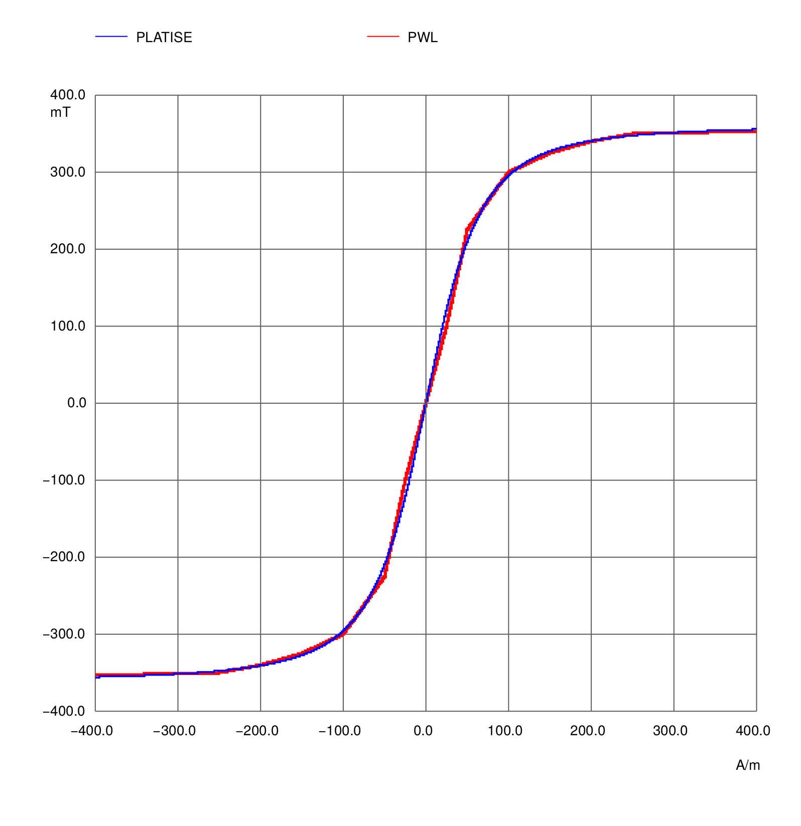
A soft-ferrite core material 26G from Iskra Feriti at T=25°C and f=5 kHz, for some hypothetical
dimensions A and len is shown below.
It is approximated with a single dipole domain (N=1) only and the result is
compared with pice-wise interpolation (PWL mode) from the points given by the data-sheet.
The current through the voltage source i(V1) represents the magnetic flux  and voltage source V1 represents the stimulus magnetomotive force
  .
.
* For easier representation we set both to 1, therefore the current i(V1)
* directly represents the B, as current is equal to a flux = B A
.param A   = 1
.param len = 1

* mode=3 selects the platise model
.model if26g core (H_array = [70] B_array = [0.361] area={A} length={len} mode=3)

* Xspice analog core model
A1 (1 0) if26g

* Magnetomotive stimulus, len=1, from -400 A to 400 A as a transient
V1 1 0 PULSE(-400 400 0 0.8ms 1ms)
Elmer FEM Usage
Platise Ferromagnetic Core has been deployed into the Elmer main development stream by calling the PlatiseFerroModel procedure. Four keywords have been introduced to be used under the Material section to specify the dipoles and control the inverse calculation.
The H-B curve, given as points from the CERN example:
has been characterized with two dipoles only, sufficiently well describing the characteristics:
PFM Dipoles Field Strength(2) = 2.63089794e2 1.96053253e4
PFM Dipoles Flux Density(2)   = 1.56587017   5.70574118e-1

! Two optional parameters
!PFM Relative Tolerance = 1e-5
!PFM Max Iterations = 100

H-B Curve = Variable "dummy"
   Procedure "MagnetoDynamics" "PlatiseFerroModel"
The two optional parameters provide additional control:
PFM Relative Tolerance = 1e-5, for instance reduces the required relative tolerance from the default 1e-6. Reduction for a decade typically reduces one iteration only inside the non-saturated area of the B-H curve and significantly more within the saturated area. Note that too low tolerance may destabilize Elmer non-linear solver resulting in increased number of iterations.
PFM Max Iterations = 100, reduces the max number of iterations from the default 1000. Typically this does not need to be controlled as under normal conditions algorithm should never reach 1000 iterations, but rather around 6 (for the default PFM Relative Tolerance of 1e-6) within non-saturated area and around 50 when it is deeply saturated.
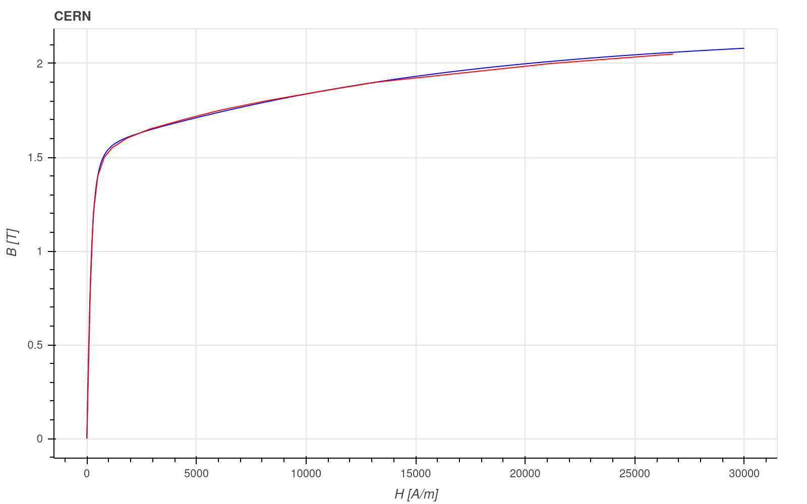
Blue line shows Platise model and red linear segments are based on original B-H points.
Complete example can be found at: https://github.com/ElmerCSC/elmer-elmag/tree/main/PlatiseFerroModel
Calculate Dipoles of your Material
Finding dipole parameters is an easy task with the help of python sci package, i.e. for the two dipoles approximation:
import numpy as np
from scipy.optimize import curve_fit

u0 = 4e-7 * np.pi

def platise_2term(H, Hm1, Bs1, Hm2, Bs2):
    return H * (np.abs(Bs1) / np.sqrt(Hm1**2 + H**2) + np.abs(Bs2) / np.sqrt(Hm2**2 + H**2) + u0)

# Provide full B-H characteristics with hysteresis within the core dictionary
# Curve fit will take the average removing the Hc.
param, param_cov = curve_fit(platise_2term, core['H'], core['B'])
param            = np.abs(param)

# To obtain results i.e. for a plot for H from -20 A/m to 20 A/m
H = np.linspace(-20, 20, 5000)
B = [platise_2term(h, *param) for h in H]
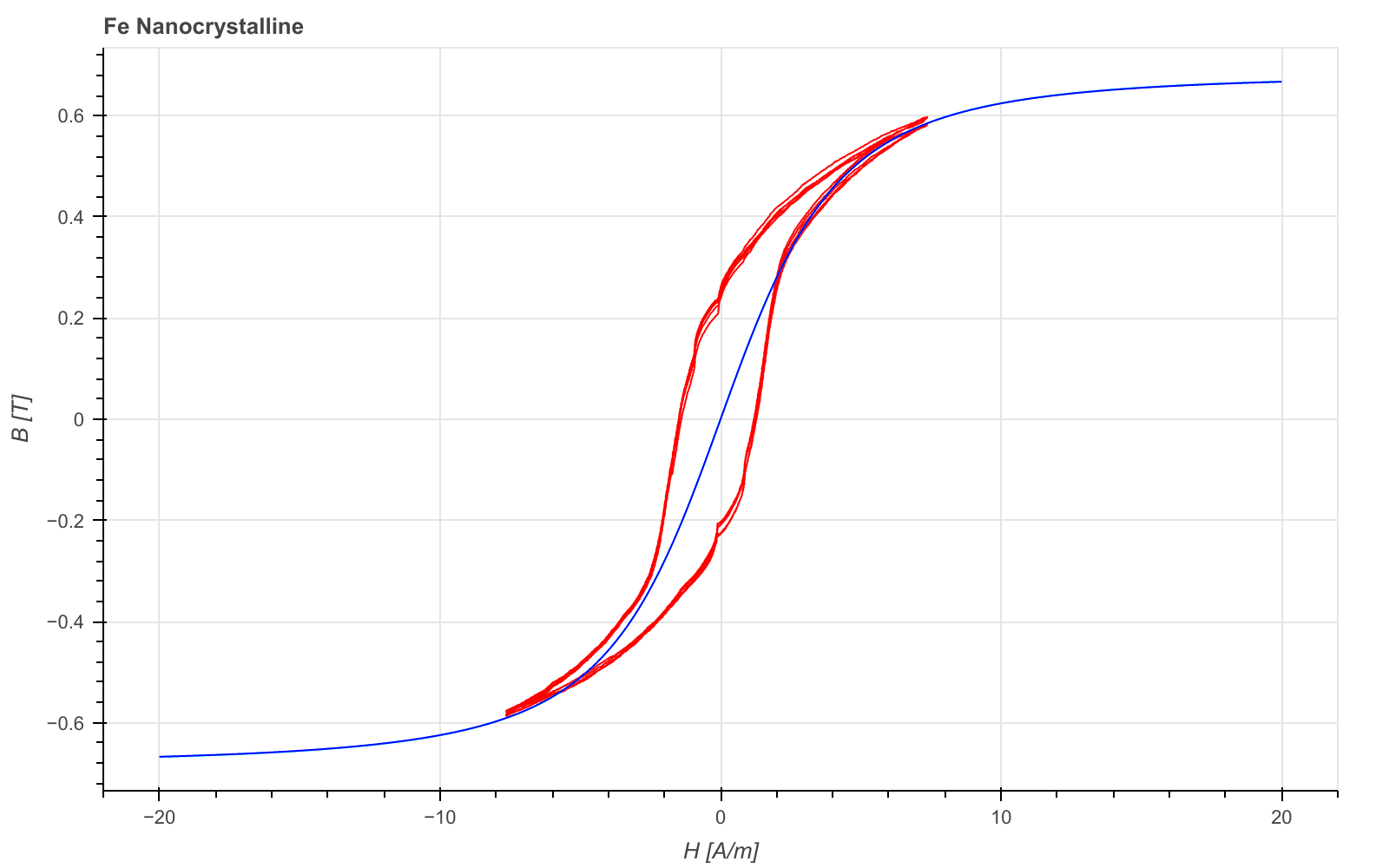
If one of the dipole is relatively small to the other or if  values are nearly equal, one dipole
approximation suffices. In the following Fe-Nanocrystalline example we can observe that the first
term of the two dipole has
values are nearly equal, one dipole
approximation suffices. In the following Fe-Nanocrystalline example we can observe that the first
term of the two dipole has  of only 1.19 uT, neglectable compared to the
  of 0.68 T. Obtained param results are the following, for:
single dipole: [4.45858037, 0.68419068]
two dipoles: [6.63222790e+00, 1.19983277e-06, 4.45119803e+00, 6.83620439e-01]
Measured B-H characteristics, in red colour, with Platise Model approximation, in blue, is shown in the following plot. Plot also shows how the Platise model smoothly extrapolates beyond the measured B-H characteristics, thus ensuring convergence even under deeply saturated conditions.
References
Platiše, “High-precision wide-bandwidth isolated current measurement in networked devices: doctoral dissertation = Natančno širokopasovno izolirano merjenje toka v omreženih napravah”, [U. Platiše], Ljubljana, 2021, pp. 25-31